Paper Dissection : Get To The Point: Summarization with Pointer-Generator Networks
In this post I will be talking about a paper on abstractive summarization which uses a generator network to generate new words when extracting summaries via a vanilla Seq2seq model with attention. This paper at the time (2017) out performed the SOTA on ROUGE by atleast 2 points.
Introduction and Motivation
Vanilla RNNs and hybrid RNNs (such as LSTMs, GRUs) have paved way for a wonderful paradigm of architectures known as Seq2seq which have provided a breakhthrough for certain tasks like abstractive summarization, machine translation etc. However, the Seq2seq architectures for summarization though better than earlier ones suffer from these known issues:
- They often while summarizing, generate factually incorrect details.
- Does not work well when there is an OOV (Out of Vocabulary) word present.
- Often repeat themselves when summarizing.
This paper, by introducing a hybrid pointer generator network along with the coverage vector has proposed an architecture which when applied to datasets CNN / Daily Mail outperformed the SOTA (in 2017) by 2 ROUGE points.
Model Architecture
There are two models described in the paper:
- Baseline Sequence to Sequence model with attention
- Pointer Generator networks.
- Sequence models with Coverage mechanism
The Coverage vector can be applied to both the models independently.
Baseline Sequence-to-sequence model with attention
This model contains a bidirectional LSTM as an encoder and a unidirectional LSTM as a decoder.
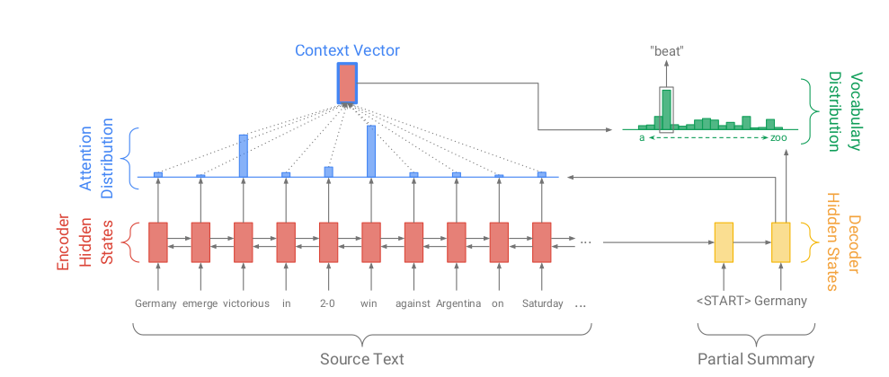
Figure 1. Baseline Architecture of Sequence to sequence model with attention
The tokens in the passage \(\boldsymbol{w}_i\) are fed one by one to the encoder (\(\boldsymbol{w}_i\) can be a Vector representation of token) and the LSTM cell outputs a sequence of hidden states \(\boldsymbol{h}_i\). And the attention distribution at a time step t represented as \(\boldsymbol{a}_t\) is calculated per the formula as in Bahdanau et al. (2015)
\[\begin{align} e_i^t &= v^t\tanh(W_hh_i+W_ss_t+b_{attn}) \tag{1} \\ a^t &= \text{softmax}(e^t) \tag{2} \end{align}\]Here, v, \(\boldsymbol{W}_h\) \(\boldsymbol{W}_s\) and \(\boldsymbol{b}_{attn}\) are all learnable parameters. Also, \(\boldsymbol{e}^t_i\) corresponds to value of attention (unbounded) that will be given to token i and \(\boldsymbol{a}_t\) provides a softmax version of it. Instead of using the final \(\boldsymbol{h}_T\) as a context vector (Where T is the last time step) the paper instead, uses the weighted sum of all the encoder hidden states as by the formula :
\[\begin{align} h_i^* &= \sum_{i} a_i^th_i \tag{3} \end{align}\]After getting the context vector, it is concatinated with the decoder hidden state at the time step t and then it will be fed through two fully connected linear layers to get a vocabulary distibution as mentioned in the top right corner of the Figure 1. Using the network trained, we can get the set of words as our summary.
\[\begin{align} P_{vocab} &= \text{softmax}(V'(V[s_t, h_t^*] + b) + b') \tag{4} \\ P(w) &= P_{vocab}(w) \tag{5} \end{align}\]And for training the network, the loss function for the timestep t can be computed as the Negative log likelihood for the target word as shown by the formula (6) and this can be summed and averaged per time step as shown by the formula (7)
\[\begin{align} loss_t &= -\log P(w_t^*) \tag{6}\\ loss &= \frac{1}{T}\sum_{t=0}^T loss_t\tag{7} \end{align}\]Pointer Generator networks
The model architecture for this network is mostly similar to the baseline with one addition where the pointer network allows for both pointing and generating new word from a fixed vocabulary according to a probability distribution.
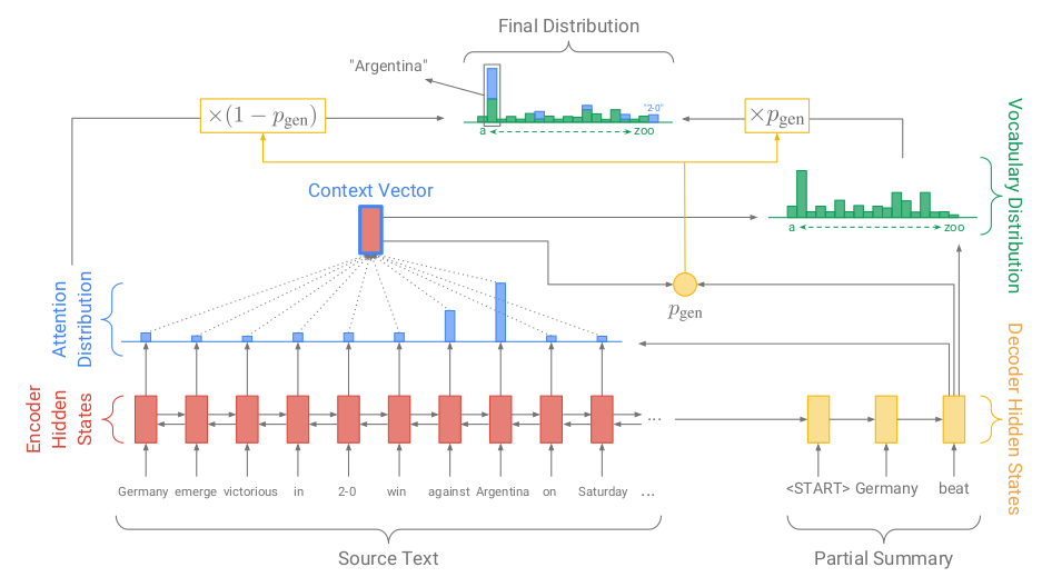
Figure 2. Pointer-generator network
For the network, the calculation of context vector \(\boldsymbol{h}_t^*\) for the decoder remains the same with the generation of \(\boldsymbol{e}_i^t\) (the activation score ) and the activation vector \(\boldsymbol{a}_t\). The probability \(\boldsymbol{p}_{gen}\), which is used as a soft switch is generated from vectors : the context vector \(\boldsymbol{h}_t\), decoder hidden state \(\boldsymbol{s}_t\) and the decoder input \(\boldsymbol{x}_t\).
\[p_{gen} = \sigma(w_{h*}^Th_t^* + w_s^Ts_t + w_x^Tx_t + b_{ptr}) \tag{8}\]Using the \(\boldsymbol{p}_{gen}\) as a switch, we try to either generate a new word by sampling \(\boldsymbol{P}_{vocab}\) (refer (4)) or copy the word by samping from the attention sequence. We will be getting a probablity distribution over the extended vocabulary where, extended vocabulary is the union of vocabulary and the words appearing in the source document. The probability distribution over the extended set :
\[P(w) = p_{gen}P_{vocab}(w) + (1 - p_{gen})\sum_{i:w_i=w}a_i^t \tag{9}\]So if the word which is being pointed to is an OOV, then the word will be copied from the attention output as \(\boldsymbol{P}_{vocab}(w)\) will be 0 and consequently, if the word does not appear in source document, then \(\boldsymbol {\sum_{i:w_i=w}a_i^t}\) be 0. For more, refer the top most graph of probabilty distribution in the figure 2. It provides an idea about the probability distribution of the words that will be generated at the decoder state by using the extended vocabulary.
The loss function is similar to the baseline Seq2seq with attention architecture as shown in the equation (6) and (7) where the \(P(w)\) is as per the latest equation (9).
Coverage mechanism
To avoid repetetion in the model output, the authors maintain that a coverage vector \(\boldsymbol{c}_t\) just helps in that. This vector maintain a sum of attention distribution over all the previous timestep. As \(\boldsymbol{c}_t\) is an unnormalized vector, it holds the degree to which the token has been attended by the model and hence \(\boldsymbol{c}_0\) is a zero vector.
\[c_t = \sum_{t'=0}^{t-1}a^{t'} \tag{10}\]This Coverage vector is used in the formula for yielding attention scores at a time step t and hence the formula of equation 1 (refer 1) changes to :
\[e_i^t = v^t\tanh(W_hh_i+W_ss_t+w_cc_t+b_{attn}) \tag{11}\]As we have to utlize this info in our training, we need to penalize if the coverage vector repeteadly attends the same tokens in different timesteps and hence we reweight the loss function with \(\boldsymbol{\lambda}\) (a hyperparameter) before adding the coverage loss to the actual loss function as provided by the equation 6 above.
\[loss_t = -\log P(w_t^*) + \sum_imin(a_i^t, c_i^t) \tag{12}\]Experiments and results
The hidden state dimension is set to 256 and the vocabulary is of 50k size for both target and source. The word embeddings are not pretrained, but are learnt from scratch in the process. Adagrad is used as the optimizer with lr = 0.15 along with gradient clipping for training. The model training also involves using early stopping on validation set. The token dimension for source is capped to 400 and the summarized version has been set to 100 tokens with 120 at test time.
Results
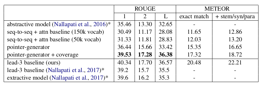
Figure 3. Summarization results in comparision to other networks
For more details on related works please refer the original paper: here .